How to Make Histogram via Google Sheets – Tutorial

Well, with work from home is becoming a norm, and professionals having to make the shift to Google Sheets, Docs. And also practically everything Drive related, if willingly or not, we must make the move now as well. In this article, we are going to talk about How to Make a Histogram via Google Sheets – Tutorial. Let’s begin!

This actually brings us to the subject of the article, that is, how can you make a histogram on Google Sheets. We actually suspect the reason you’re here is that you have realized or discovered that things work a little differently on Google Sheets. If we as compare to the way they did with Excel or whatever software you used before for number crunching and analyzing data. One thing you can make sure of is that Google Sheets is very easy to use and navigate as well.

What is the Normal Distribution Curve?

The normal distribution curve is basically a graphical representation of the normal distribution theorem. That says that “…the averages of random variables independently drawn from independent distributions converge in distribution to the normal. That is, become normally distributed whenever the number of random variables is sufficiently large”.

Bit of a mouthful, but in life, the data converges around the mean (average) along with no skew to the left or right. It actually means we know the probability of how many values occurred close to the mean.

We expect 68% of values in order to fall within one normal deviation of the mean, and 95% to fall within two normal deviations. Values outside two average deviations are actually considered outliers.

How to Make Histogram via Google Sheets

The premise is more or less the same along with Google Sheets just like it was for Excel. You guys need to apply the relevant cell formula in order to manipulate data and calculate numbers. If you want your chart to be really thorough. The next steps will elaborate on how you can add a Histogram chart in google sheets.

Create a data range

A data range is basically a cell grid that you create along with relevant numeric information that is to be represented on the Histogram. For the purpose of this article, we have also created two data cells that range between values 43 and 95. Have a look at our data range allocated to columns A and B.

We are using these columns in order to create our Histogram. You can also create your Histogram using this one or also use data of your own.

How can you add a Histogram Chart | Histogram via Google Sheets

• First, you need to open a blank spreadsheet in Google Sheets through tapping the blank icon.
• Then you guys will now be looking at a blank spreadsheet. Now from the menu panel, tap on Insert.
• From the menu that opens, you need to tap on Chart.
• Now you guys will see a Chart editor open next towards the right side. From the Setup tab, tap on the dropdown menu for Chart Type.
• Scroll towards the end of the menu until you reach the Other option where you guys will see an option for a Histogram chart, tap on it.

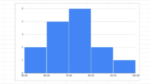
The histogram chart is added to your sheet. It should look just the same as this image:

How can you edit the Histogram chart via Setup Tab

The Setup Tab is where you guys will find the options and settings that are needed to add the applicable information from the columns to the chart. This is actually the place where you set the base for the histogram. Basically, the Setup Tab gives you permission to incorporate the data sets into it.

• For any type of editing activity, you guys will have to tap on the three-dot menu icon on the top right section of the chart. And then tap on select the Edit chart option.
• When you do that, then the Chart Editor will pop up towards the right side of the screen. There you will see two tabs, Setup and Customize as well. Tap on Setup.
• Now within the Setup tab in the Chart Editor, you also have to set the data range for the chart. If you want to do this, then tap on the Select Data Range icon.
• Now, you can select one of two formats. Either club both the columns together in order to form a single panel chart. In that case add all the cells (A1: B15) in one range.
• Or, you guys can also create another range for the next column as well.

Then your Histogram will look like this:

• You guys can also create one entire set of series which would then be A1: B15 or you can also separate the two columns too.
• If you select to club all the columns into one series, then the histogram chart won’t look and different from what it was before.
• Now in the last section of the Setup Tab, you guys will see the following options along with checkboxes. You can also choose them if you wish to incorporate those settings in the chart.

How can you edit the Histogram chart via Customize Tab | Histogram via Google Sheets

• Well, in the customize tab, you can change the look and feel as well as add features to your histogram too.
• In the Chart Style section, you can also change the font, background, and chart border color of the chart as well.
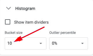
• Next, you can also set the bucket size of the chart in case you want to increase it. Sheets offers a bucket size of more than 50. Well, you can also show the x-axis in outliers.
• In the next section, you can also name your chart and change the font and font size as well.
• When you tap on the chart title, then you can name every axis and also give subtitles should you wish.
• Also, you can even set the position of the legend.
• The next sections will give you permission to customize the font of the text that represents both of the axes. You can select to forgot this unless you have to follow a design guideline actually. The same applies to gridlines and ticks as well. Simply tap on the arrow for each and every section to open them and apply whichever settings you guys want.

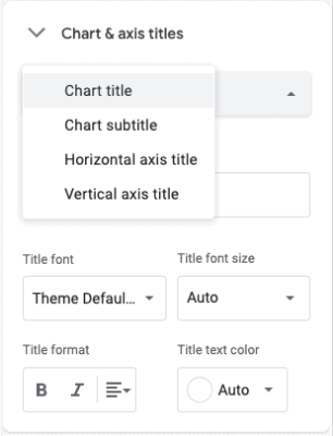
Chart & axis titles | Histogram via Google Sheets

This submenu is really helpful for adjusting how the chart title, chart subtitle, horizontal axis title, and also vertical axis title display. You can also set the following for each:

• Text: The selected feature display text. such as, the chart title might read “Histogram of Age” or “Respondent Age Histogram.”
• Font: choose the font-family
• Font Size: Select how big this text element displays.
• Format: Set bold, italics, and alignment as well.
• Text Color: Select the color for the selected text.

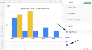
Series | Histogram via Google Sheets

This tab basically lets you select the bar color for each and every series in your histogram. It’s particularly useful if you have a histogram comparing multiple series actually.

You have to djust the series color along with the following steps:

• Choose the series that you want to adjust from the main drop menu (top black arrow).
• Then choose the color you want to represent the series from the “Color” drop menu (bottom black arrow).

Legend | Histogram via Google Sheets

The “Legend” submenu actually lets you make adjustments to its namesake (in the above blue rectangle). The options basically make the following adjustments, have a look:

• Position: This moves the legend to the top, bottom, left, or also right relative to the graph. Choose “None” to delete the legend or “Inside” to move the legend on top of the chart as well.
• Legend font: It changes the display font for the legend.
• Legend font-size: It adjusts the font size for the legend actually.
• Text color: Set the legend’s text color as well.
• Then legend format: Bold or italicize the legend along with these options.

Horizontal axis & Vertical axis | Histogram via Google Sheets

These two options sections basically serve the same purpose, however for the horizontal axis and vertical axis actually.

These options basically let you adjust the range of the graph that can provide important context to a histogram. Plus, they also let you change the appearance of the axis information.

Min and Max (Setting the Range): These are very useful options in order to add context to a graph. You can also select both the lowest (min) and highest (max) value represented in the histogram.

The other options also relate in order to formatting the axis text:

• Label font: It changes the font for the axis.
• Label font size: Force the text size actually
• Text color: It basically change the text color.
• Label format: Bold or italicize the text as well.
• Slant labels: Display the axis labels on an angle actually. This can make a crowded graph really easy to read.

Conclusion

Alright, That was all Folks! I hope you guys like this article and also find it helpful to you. Give us your feedback on it. Also if you guys have further queries and issues related to this article. Then let us know in the comments section below. We will get back to you shortly.

Have a Great Day!

Also See: How to Highlight Duplicates in Google Sheets